12 Data processing
This chapter gives a little more detail on the steps followed in processing the data before aggregation.
12.1 Outlier treatment
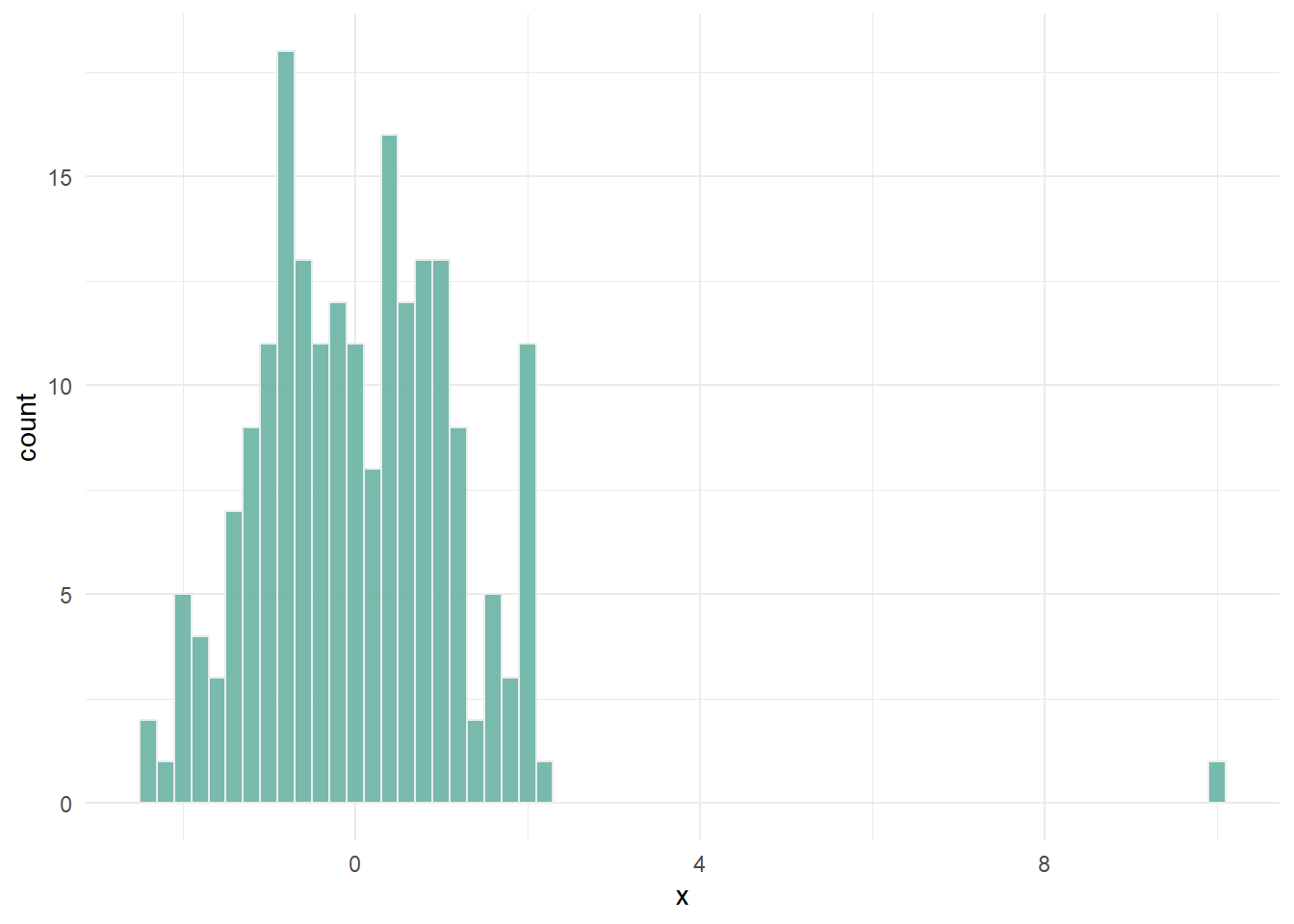
Outliers are roughly defined as data points that don’t fit the rest of the distribution of the indicator. Consider the artificial example below:
Outliers can exist because of errors in measurement and data processing, and should always be double-checked. But often, they are simply a reflection of reality. Outliers and skewed distributions are common in socio-economic variables.
Outlier treatment is the process of altering indicator values to improve their statistical properties, mainly for the purposes of aggregation. The reason why we may want to treat outliers is that in composite indicators, before aggregating we typically normalise the data by scaling it onto a common range (e.g. 0-100). When an indicator has outlying values, as in the example above, the outlier will “dominate” the scale and result in a large part of the indicator scale being empty.
Typically the implication is that the large majority of points (Admin-2 regions here) end up with either a very low score (or high, depending on which side the outlier is on), except for the outlier. This can turn the indicator into a trivial measure of “is the observation the outlying region or not?”, which is not usually what we want to measure.
Consider that data treatment is simply another assumption in a statistical process. Like any other step or assumption though, any data treatment should be carefully recorded and its implications understood.
The A2SIT app has an outlier treatment algorithm which treats outliers automatically when the results are calculated. The methodology follows that used by the European Commission, among others, and is as follows.
For each indicator separately:
- Check skew and kurtosis value
- If absolute skew is greater than 2 AND kurtosis is greater than 3.5:
- Successively Winsorise up to a maximum of five points. If either skew or kurtosis goes below thresholds, stop. If after reaching the maximum number of points, both thresholds are still exceeded, then:
- Return the indicator to its original state, and perform a modified log transformation.
- If the indicator does not exceed both thresholds, leave it untreated.
Here, the skew and kurtosis thresholds are used as simple indicators of distributions with outliers.
Winsorisation involves reassigning outlying points to the next highest or lowest point, depending on the direction of the outlier. In the example above, this would involve taking the outlier with a value of 10, and reassigning it to the maximum value of the observed points except that one. This treatment can be applied iteratively, in case of multiple outliers.
The log transformation involves applying a scaled log-transformation that reshapes the entire distribution. It is most suitable for naturally skewed distributions such as log-normal distributions. Since the direction of skew can be either positive or negative, the transformation adapts accordingly. For positively-skewed indicators:
\[ x' = \log(x-\min(x) + a)\\ \text{where:} \;\;\; a = 0.01(\max(x)-\min(x))` \]
Else if the skew is negative:
\[ x' = -\log(\max(x) + a - x)\\ \]
This transformation is effectively a log transformation with a small shift, which ensures that negative values can also be transformed.
12.2 Normalisation
The normalisation step aims to bring indicators onto a common scale, which makes them comparable for the purposes of aggregation. The A2SIT app uses the common “min-max” approach, which simply rescales each indicator onto the \([1, 100]\) interval:
\[ x' = \frac{ x - x_{\text{min}} }{ x_{\text{max}} - x_{\text{min}} } \times (100-1) + 1\]
where \(x'\) is the normalised indicator value. This means that the lowest observed value of each indicator, over all Admin-2 regions, will get a score of 1, and the highest observed value will get a score of 100.
The min-max method is simple to understand and communicate. We set the lower bound at 1 to acknowledge the fact that the minimum value does not imply a true zero in that indicator (i.e. there is not an absence of severity).
Note that the app additionally uses an ex-post rescaling onto a 1-5 categorical scale. This is explained more in the following chapter.
12.3 COINr implementation
The relevant code for these steps can be found in the f_build_index() function, which is on GitHub here. In COINr, the code looks like this:
max_winsorisation <- 5
skew_thresh <- 2
kurt_thresh <- 3.5

# treat outliers
coin <- COINr::qTreat(
  coin, dset = "Raw",
  winmax = max_winsorisation,
  skew_thresh = skew_thresh,
  kurt_thresh = kurt_thresh,
  f2 = "log_CT_plus")

# normalise to [1, 100]: otherwise if we have zeros can't use geometric mean
coin <- COINr::Normalise(
  coin,
  dset = "Treated",
  global_specs = list(f_n = "n_minmax",
                      f_n_para = list(l_u = c(1, 100)))
)